Atomic physics
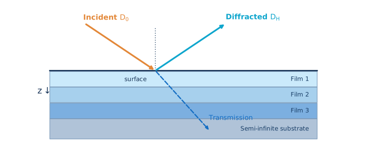
CIF geometry, structure factors, anomalous dispersion, susceptibility and the diffraction vector.
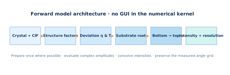
A developer-level guide to coherent X-ray diffraction from crystalline multilayers: from atomic scattering and susceptibility to Takagi–Taupin, Riccati propagation, the Bartels recursion and a verifiable numerical implementation.
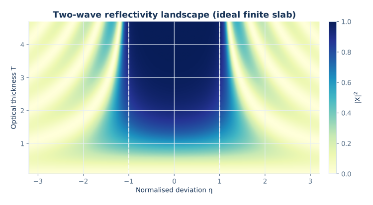
Exact two-wave slab solution · Optical thickness T versus detuning η
This is a detailed theory-to-code pathway for high-resolution coupled 2θ–ω X-ray diffraction scans of layered crystals. Unlike a textbook overview that ends at Bragg’s law, we follow complex amplitudes all the way from material data to a detector-ready intensity.
CIF geometry, structure factors, anomalous dispersion, susceptibility and the diffraction vector.
Takagi–Taupin coupling, normalized Riccati equation, branch choice and transfer matrices.
Substrate boundary conditions, reverse layer recursion, strain and coherent attenuation.
Angular convolution, numerical resolution, reproducible tests and physically meaningful fitting.
X-ray wavelength; Å for crystal data.
θ, 2θSample angle and detector angle; convert degrees → radians before trig functions.
H = (hkl)Reciprocal lattice vector; H is not simply a Cartesian direction in non-cubic crystals.
χ0, χ±HComplex Fourier components of electric susceptibility.
D0, DHComplex transmitted and diffracted wave envelopes.
η, T, XNormalized detuning, optical thickness and amplitude ratio within a declared convention.
γ0, γHProjections of propagation directions on the surface normal.
DWCoherent amplitude reduction; distinguish microscopic Debye–Waller from phenomenological damage models.
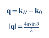
An X-ray plane wave produces an elastically scattered wave whose phase depends on the scattering position. The momentum-transfer vector is the difference between the scattered and incident wave vectors; for elastic scattering both have magnitude k = 2π/λ.
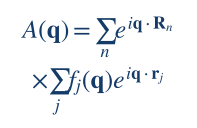
For atoms at positions rj within unit cells translated by Rn, the coherent scattering amplitude factors into a lattice term and an atomic basis term:
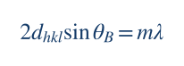
Constructive interference occurs when the scattering vector meets a reciprocal lattice point, q = H = ha* + kb* + lc*. In a symmetric scan, |q| = 4π sin θ / λ and |H| = 2π/dhkl; equating them gives Bragg’s law.
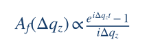
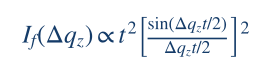
A uniform, sufficiently thin film of thickness t accumulates an extra phase Δqzz away from the exact reciprocal-lattice condition. Integrating over depth gives the familiar thickness-amplitude formula, and the squared modulus produces the sinc-shaped envelope.
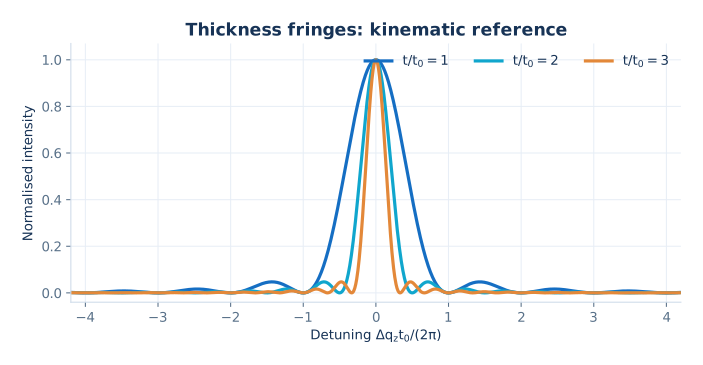
The plot is useful for intuition: thicker films give narrower main peaks and more closely spaced fringes. But it ignores multiple scattering, extinction, refraction and strong substrate reflections. Near an intense Bragg reflection, adding separate intensities for layers is fundamentally wrong; the correct object to propagate is the complex amplitude.
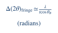
This is a kinematic estimate in radians for the 2θ axis, not a substitute for numerical convergence tests.
Every reflection depends on the atom positions, occupancies, wavelength and atomic form factors. A useful crystallographic implementation separates these inputs from thickness and other sample-stack parameters. The scattering factor includes non-resonant and anomalous terms:
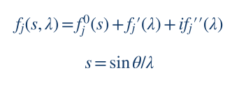
The crystal structure factor for reciprocal vector H = (hkl) is a coherent sum over atoms in the unit cell. Occupancy oj, Cartesian-equivalent fractional coordinates and atomic displacement factors all enter before the dynamical solver:

Here Wj is the crystallographic displacement exponent. For a compound or alloy, occupancies must follow the modelled composition. For a monoclinic or hexagonal crystal, use the full unit-cell metric to compute interplanar distances and the scattering direction; do not use cubic-only shortcuts.
The connection to Maxwell’s wave equation is made through the Fourier components of the complex electric susceptibility:
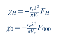
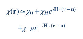
Here re is the classical electron radius, Vc the unit-cell volume and F000 forward scattering. Under the convention shown, χ0 produces refraction and absorption; χH and χ−H provide coherent Bragg coupling.
For many trial thicknesses or strain profiles of the same material, the undistorted atomic positions and scattering tables can be reused. However, dhkl, Bragg geometry, wavelength-dependent factors and any angle-dependent scattering approximation must be invalidated when their physical inputs change. The MROX Studio 41 manual distinguishes full and fast structure-factor evaluation; the latter must still be keyed by the relevant per-layer Bragg condition.
When a wave repeatedly scatters between the transmitted and diffracted channels, the fields are coupled. Begin with the scalar Helmholtz equation for one selected polarization (a Maxwell/vector treatment is required when the scalar approximation fails):
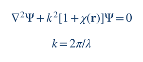
Close to a single reciprocal-lattice vector H, retain the average and two resonant harmonics of the susceptibility. Distortion is represented by a displacement field u(r) which modulates the lattice phase:
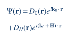
Decompose the internal field into two nearly resonant carriers with slowly varying envelopes, keeping the transmitted and Bragg-diffracted beams explicitly:
In a generic sign convention, the first-order coupled system has the structure:
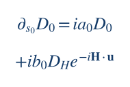
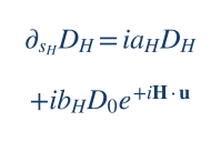
The coefficients a0, aH contain refraction and deviation from exact Bragg diffraction, while b0, bH contain the Fourier susceptibilities, polarization factor and geometry. The exact assignment of χH versus χ−H and displacement-phase signs follows the chosen Fourier convention: derive both equations consistently rather than mixing sources.
For a laterally uniform stratified crystal, all material properties depend on depth only. The coupled PDEs then reduce to ordinary differential equations. This 1D reduction enables exact constant-slab propagation and is the relevant model for the present 2θ–ω page.
A consistent change of coordinate, phase and amplitude normalization transforms the two-wave system into a simple canonical pair. This is an explicitly declared mathematical convention, not a claim that the legacy MROX variable Xt has exactly these signs.
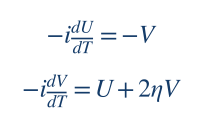
Introduce the normalized ratio X(T) = V(T)/U(T). Differentiate this quotient:
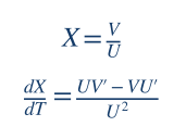
Using U′ = −iV and V′ = iU + 2iηV, we obtain −iX′ = (U² + 2ηUV + V²)/U². Hence:
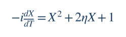
Notice that absolute phase and intensity scale have disappeared, but coherent interference is retained because X remains complex. This reduction is the mathematical basis for efficient amplitude-ratio recursions in 1D Bragg diffraction.
From the canonical relation U′ = −iV, we have X = iU′/U. Substitution into the Riccati equation cancels the quadratic derivative terms and produces a second-order linear equation:
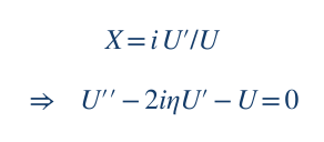
Solving this linear equation and forming V/U must agree with a direct Riccati solver and a 2×2 matrix exponential. That three-way equivalence is a valuable unit test.
For constant η, the two stationary solutions are the roots of the Riccati quadratic:
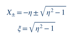
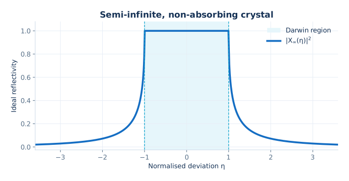
For real η without absorption, the interval |η| < 1 is the ideal Darwin region: the square root is imaginary and strong coupling occurs. Outside it, the roots are real. In an absorbing crystal, η and the square root are complex; the physically acceptable root is selected by analytic continuation and the non-growing wave condition, not by an arbitrary sign test alone.
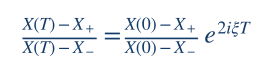
This exact expression propagates a starting ratio through a homogeneous slab. It is compact but not always the most stable numerical representation: close to a root, both numerator and denominator may become small, and exponential factors can overflow for thick or absorbing layers. Matrix/ratio/scattering formulations should be cross-checked.
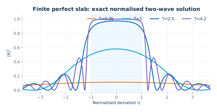
Computed from the exact dimensionless two-wave slab transfer matrix with Xin = 0, not from a fitted experimental diffractogram.
Write the canonical two-wave system as Y′ = A Y where Y = (U, V)T and A is constant inside a homogeneous slab:
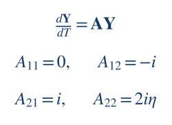
Then Yout = exp(AΔT)Yin. The matrix explicitly includes coherent coupling, so no interference phases need to be approximated by hand. Instead of propagating arbitrarily scaled fields, form their ratio. Any 2×2 linear transform induces the fractional linear (Möbius) map:
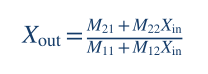
The key computational advantage is that Xout depends only on the starting ratio and the slab parameters, so the whole stack can be traversed without storing absolute fields at every interface. However, a singular or near-zero denominator must be handled carefully, especially for absorbing and very thick slabs.
import numpy as np

def propagate(x_in, eta, T):
    """Exact normalized two-wave transfer; not production MROX physics."""
    eta = complex(eta)
    s = np.sqrt(1.0 - eta*eta)
    h = T if abs(s) < 1e-10 else np.sinh(s*T)/s
    c = np.cosh(s*T)
    # Overall exp(i*eta*T) cancels from the complex ratio.
    m11 = c - 1j*eta*h
    m12 = -1j*h
    m21 = 1j*h
    m22 = c + 1j*eta*h
    return (m21 + m22*x_in)/(m11 + m12*x_in)

# Two-beam, lossless finite slab; dimensionless detuning.
print(abs(propagate(0j, eta=0., T=1.5))**2)
Why does the code use hyperbolic functions? The trace-shifted matrix A − iηI squares to (1−η²)I. Therefore the matrix exponential is a combination of cosh(sT) and sinh(sT)/s, where s = √(1−η²). The s → 0 limit should be handled analytically as sinh(sT)/s → T.
The bottom of a Bragg stack is usually treated as a semi-infinite crystal. One does not prescribe an unrelated diffracted wave arriving from infinite depth. Instead, choose the eigenmode that meets the physically appropriate boundedness condition at depth, including absorption and the direction of energy flow.
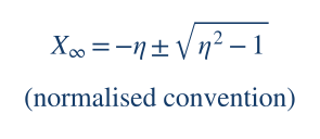
That expression shows the canonical roots. In the MROX Studio 41 implementation described in the supplied manual, the substrate ratio is written in a different normalization as Xt = η ∓ √(η²−1). The change of sign is not a bug by itself; it is a change of convention. A developer must transform η, T and X together, then verify the predicted observable.
In the ideal nonabsorbing, symmetric and properly flux-normalized case, the substrate intensity shows the Darwin plateau. Within the two-wave framework a common surface intensity expression includes the structure-factor ratio:
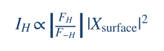
Its flat high-reflectivity region is a defining distinction from the thin-crystal kinematical approximation. In real XRD data the plateau is modified by absorption, asymmetric geometry, polarization, instrumental response and crystal perfection.
Bartels, Hornstra and Lobeek showed how dynamical diffraction from complex multilayers can be computed by a recursive amplitude-ratio treatment derived from Takagi–Taupin equations. The underlying physical boundary condition is known at the semi-infinite substrate, so the recursion proceeds upward through the films.
For each homogeneous layer j and each angular point, prepare its detuning ηj, dynamical thickness Tj, complex coupling factors and the ratio arriving from the layer below. The supplied MROX Studio 41 manual documents this specific Bartels-family algebra:
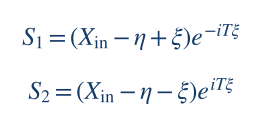
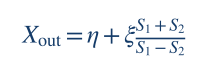
The dynamical thickness in that documented implementation can be written as
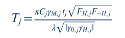
where γM = re λ²/(π Vc); tj and λ must use identical length units (for example, 1 nm = 10 Å). Polarization enters through C; γ0 and γH contain the beam/surface geometry. A characteristic dynamical coupling length is proportional to:
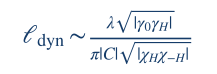
The proportionality and exact “extinction length” definition vary between authors and geometry conventions. The useful interpretation is universal: the larger the coupling and the thicker the crystal relative to its dynamical length scale, the less reliable the single-scattering approximation.
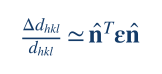
A spatially varying displacement field causes a phase shift H·u(z) in the diffracted wave and changes the local condition for Bragg diffraction. At first order, the relative change in interplanar spacing is the strain tensor projected along the actual reciprocal-space normal:
Differentiate Bragg’s law at fixed wavelength to obtain the angular shift. When plotting a 2θ scan, the factor of two comes from the detector axis:
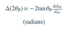
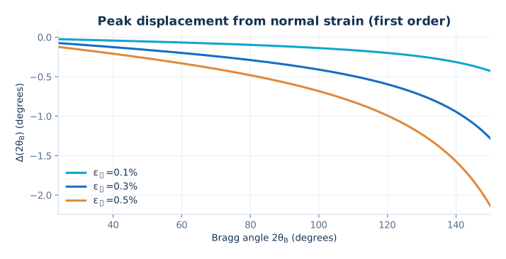
A positive normal strain increases the plane spacing, shifting the reflection to smaller 2θ; a contraction shifts it upward. The plot shows the first-order rule for several example strain values. At larger strain or near complex material geometries, update the complete lattice metric instead of relying on the derivative.
The in-plane strain of an epitaxial film can be constrained by the substrate lattice; the out-of-plane strain follows from the elastic tensor and the appropriate free-surface stress conditions. In tensor/Voigt notation:
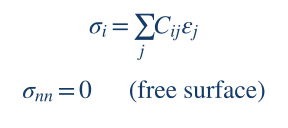
For cubic (001) layers, textbook biaxial relations are often sufficient, but they do not generalise blindly to monoclinic β-Ga₂O₃, non-cubic cuts or arbitrary off-axis reflections. A robust solver builds the direct and reciprocal lattice bases from the CIF, rotates the elastic stiffness tensor into sample coordinates, then solves the plane-stress conditions.
Thermal motion and static disorder make the atomic scattering phases fluctuate. For a zero-mean Gaussian displacement vector with covariance tensor U, the coherent average scattering amplitude at reciprocal vector H is:
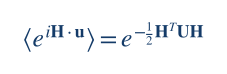
For an isotropic displacement along H, this reduces to exp(−½|H|²σu²). Intensity is reduced by the squared modulus, not by the same factor again unless that is how the chosen parameter is explicitly defined.
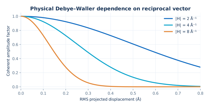
This dependence on |H|² is the key microscopic prediction: higher-order Bragg reflections may be more sensitive to displacement disorder. It is not equivalent to an arbitrary empirical attenuation that happens to be called “DW”. A fitted Debye–Waller-like damage parameter can also absorb mosaicity, inhomogeneity or instrumental effects if the model is insufficiently constrained.
In standard crystallographic displacement theory the Debye–Waller factor damps nonzero reciprocal harmonics FH but does not reduce F000 by the same mechanism, because H=0 makes the phase fluctuation vanish. The supplied manual flags that the examined MROX Studio 41 implementation multiplies FH, F−H and F000 by a layer DW factor. It records this as a physics question for testing, not as a validated microscopic identity.
Ion implantation changes lattice parameter, static disorder and sometimes the coherent diffracting fraction as a function of depth. A piecewise-constant discretisation approximates continuous profiles by many small slabs, each with its own strain, atomic parameters and coherent attenuation.
The supplied manual describes a sum of asymmetric Gaussian strain components, with a potentially different width on each side of the maximum:
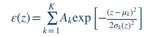
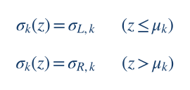
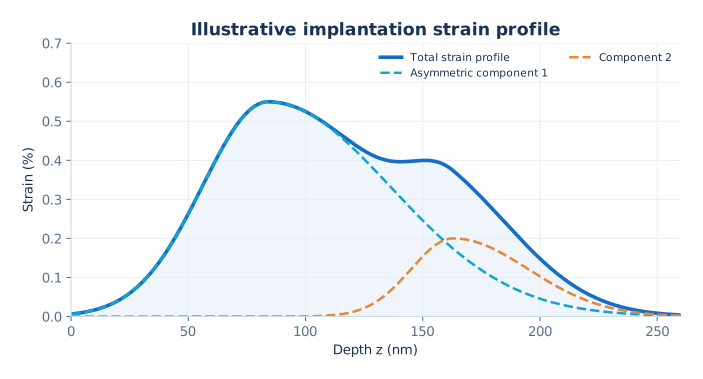
The amplitudes Ak in that model are expressed in percent strain; the centres and widths are distances. Convert displayed FWHM values to Gaussian standard deviations using FWHM = 2√(2 ln 2) σ. When discretising, take values consistently at slab midpoints or use slab-average integration if higher accuracy is required.
To maintain physical comparability under refinement, changing the slab step Δz must leave the total affected thickness and continuous profile unchanged. Shorten the final slab if necessary rather than silently rounding the thickness upward. Check the complete stack after applying a profile: the material, strain, thickness and DW of unrelated layers must remain unchanged.
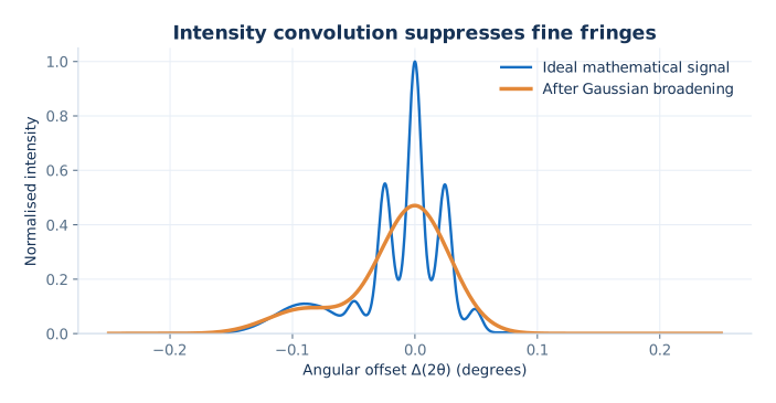
The two-wave result describes an ideal coherent diffraction intensity. The experimental detector sees a response affected by source spectrum, divergence, angular acceptance and background. Typically the instrument acts on intensity after coherent wave propagation:
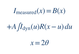
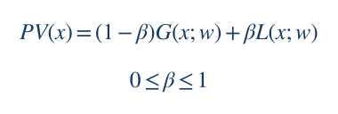
A widely used parameterisation of an angular response is the pseudo-Voigt function, mixing Gaussian and Lorentzian line shapes. Define both components with the same FWHM w and each normalised to unit integrated area:
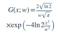
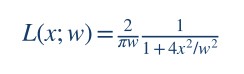
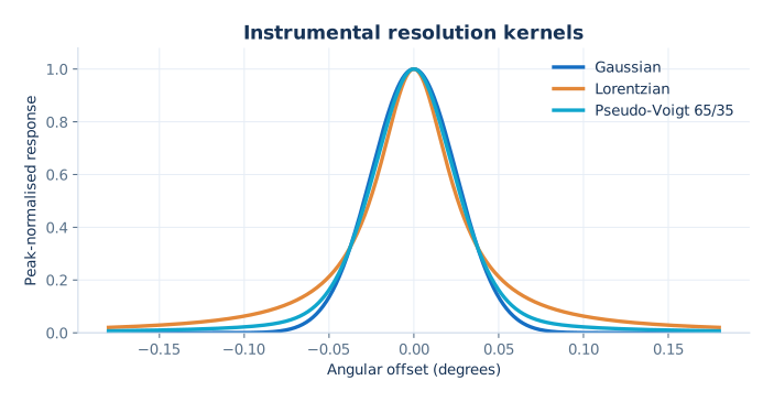
Within a single two-wave scalar approximation, a common polarisation coupling factor is Cσ = 1 or Cπ = cos(2θB). Some intensity-only codes use its absolute value inside their coupling normalisation; if this is done, keep phase conventions consistent throughout propagation.
The Cu Kα₁ and Kα₂ photons have different wavelengths. Therefore, their peak positions must be calculated from their respective wavelengths via Bragg’s law, and the intensities added incoherently according to the source spectrum and optical selection. Reusing a single simulated profile and applying an arbitrary angular translation is only an approximation whose accuracy depends on scan range and material.
The supplied manual separately describes a legacy-inspired empirical model in which Gaussian smoothing increases with angular distance from the substrate Bragg position. It is a useful fit model but is not a first-principles model of every diffractometer:
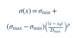
Here x = 2θ, Dmax = maxx|x−xB|, and the width interpolates between σmin and σmax with exponent p > 0. Because each output point has its own kernel width, ordinary stationary convolution is not exactly the same operation.
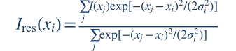
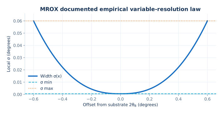
The displayed discrete version is a locally normalised Gaussian weighted average; it preserves a constant signal. For uneven angular grids, sampling density must be accounted for with integration/quadrature weights if one wants a proper continuous integral approximation. For a scan with very small σ compared with the angular step, oversampling is needed before claiming accurate sub-step broadening.
For someone developing a new program, it helps to separate a minimal mathematically verifiable solver from a fully physical crystal simulator. The first proves that the amplitude algebra is consistent; the second adds material, geometry, boundary conditions and instrument physics. Implement these layers in this order.
Write down the time dependence (e−iωt or e+iωt), reciprocal-space Fourier sign, direction of depth, orientation of surface normal, transmitted/diffracted amplitude normalisation and branch criteria. Fix a single meaning for η, T and X.
Implement Y′ = AY and the Möbius map first. Compare matrix propagation with the analytic Riccati formula, including T→0, η=±1 and long slabs. The included riccati_reference.py performs some of these tests.
Read CIF unit-cell parameters, symmetry and fractional coordinates; form the reciprocal metric, dhkl, Vc and all relevant complex F. Verify the results against known reference reflections before entering the TT code.
Calculate susceptibilities and the geometry-dependent coefficients at each angular point. Transform into the exact normalized variables of the chosen recurrence. Establish and record how the flux factor converts surface X into measured reflectivity.
Use radiation/decay conditions and analytic continuation under absorption. Test continuity as detuning passes through the Darwin edges and compare against independently published perfect-crystal results.
Recurse bottom-to-top, preserving complex phases. Update the full lattice metric under strain; discretise profiles by depth while retaining physical thickness. Separate microscopic Debye–Waller from empirical coherent attenuation.
Apply source spectrum, polarisation, calibrated resolution, background and any explicit angular-zero correction. Preserve the original experimental angular grid; do not move measured points to improve agreement.
Use a pure function simulate(parameters, angles) that does not mutate UI state or files. Cache by dependencies, not by convenient but incomplete labels. Let fitting algorithms, uncertainties and optional Bayesian inference call the same forward engine.
All visual assets are supplied locally. The mathematical demonstration code is open for study and modification; it is not a reconstructed MROX production solver and cannot predict a specific material before susceptibility, geometry and boundary conditions are implemented.
A simulated rocking curve can look beautiful while being physically wrong. The following tests should be automatic and run when any sign convention, absorption formula or propagation kernel changes.
| Test | Expected property | What it catches |
|---|---|---|
| Zero slab thickness | Xout → Xin as T → 0. | Incorrect transfer order, signs and singular limits. |
| Analytic Riccati vs matrix | Same complex amplitude in the same declared convention. | Formula transpositions and eigenvalue errors. |
| Ideal finite slab | Finite, nonnegative intensity; flux conservation in lossless normalised cases. | Wrong intensity factor or unstable propagation. |
| Substrate branch | Physically decaying/causal solution with smooth absorption limit. | Wrong square-root sheet and unphysical gain. |
| Identical adjacent layers | Splitting a homogeneous slab must not change reflectivity. | Incorrect interface and matrix composition. |
| Zero diffraction coupling | Bragg-reflected amplitude tends to zero appropriately. | Spurious kinematic/dynamical mixing. |
| Angular grid refinement | Curves and peak positions converge under halving angular spacing. | Aliased fringe periods and false peak maxima. |
| Depth-grid refinement | Profiled-stack reflectivity converges as Δz is halved. | Under-resolved implantation gradients. |
| Instrument OFF | Raw coherent intensity unchanged. | Hidden filtering and double convolution. |
| Constant-input filter | Local normalised Gaussian returns the same constant. | Bad boundary normalisation. |
| Absorption and anomalies | No unphysical amplification; complex F−H handled independently. | Conjugation assumptions and branch errors. |
| Strain sign and units | Expanded spacing shifts the ideal peak towards lower 2θ. | Percent/fraction errors and flipped geometry. |
A useful slab-grid convergence metric is:
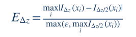
Here the two curves are evaluated on the same angular points and with the same underlying continuous strain/DW profile. Relative to full-scale maximum intensity, EΔz is a reproducible discretisation estimate, though weak features may need a log-intensity or local criterion.
Complex square roots change sign across branch cuts. Track the physical eigenmode continuously, with an explicit absorption sign convention.
Transfer matrices can overflow or lose significant digits for thick layers. Consider normalised Möbius maps and scattering matrices.
The fractional transform can become ill-conditioned even when the physical reflectivity remains finite. Add tests and safe alternative forms.
Sub-step fringes are not accurately recovered by a smoothing filter. Oversample and integrate appropriately.
As an example, the supplied manual records a deterministic objective combining robust logarithmic error, overall intensity correlation and first-difference correlation:
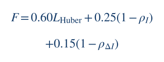
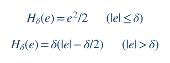
This is a project-specific optimisation score, not a normalised probabilistic likelihood. If a new solver reports Bayesian credible intervals, it must instead specify a statistical residual model and prior. For independent Gaussian log-intensity errors with common scale σ, the log-likelihood has the generic form:
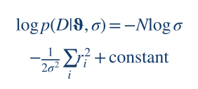
Instrumental width, strain, roughness/damage and thickness can be highly correlated when fitting only one symmetric reflection. Confidence in extracted physical parameters is improved by independent measurements, more reflections, explicit uncertainty analysis and robustness across initial guesses.
Bragg/kinematic relations, susceptibility mapping under the stated sign convention, the dimensionless Riccati identity, constant-slab matrix propagation and the figures computed from those equations. The supplied reference Python script checks the analytic/matrix identity numerically.
Actual MROX Studio 41 material-specific numerical outputs, branch mapping between its Xt and canonical X, the phenomenological DW treatment of F000, resolution calibration and any inferred sample-specific strain or disorder.
The supplied manual explicitly describes a static code audit rather than experimental or MATLAB runtime validation. The present page follows that distinction. It explains scientific methods openly and teaches reproducible mathematics; it does not publish unverifiable experimental results or claim identity with proprietary algorithms solely on the basis of similar-looking expressions.
Foundational references for independent readers who want to inspect derivations and build their own software. DOI links lead to the publishers’ original records.
CONTINUE EXPLORING
Explore how XRD/XRR modelling is used in real scientific publications, or study the reproducible example code included with this page.